7. Coherent Multidimensional Spectroscopy - The CMDS Class

Simulating two-dimensional (2D) spectra is generally difficult. You could try to manually simulate 2D spectra using the toolbox. In that case, you would need to write loops over simulations, change external field delays and phases, perform phase cycling, and more. To simplify this repetitive work that is similar for all multidimensional spectroscopy experiments, we have included the CMDS (Coherent Multidimensional Spectroscopy) class. This class takes a different place in the toolbox structure in that it takes an instant of the System class and performs multiple simulations using different interpulse parameters within a multipulse external light field. To use the CMDS class you have to define a System object in the usual way. In our simple example we will just have a single qbit on which we perform a population-based 2D experiment where we calculate the photon echo signal contribution by a three-pulse sequence.

1 2 3 4 5 6 7 8 9 10 11 12 13

s = System; s.lso = true;  %use the lindblad superoperator gaps = [2.0*s.evtoau]; a = Nlevel(gaps); a.setDipole([1 0], 1); s.addEntity(a, 'molecule'); s.addDissipation('molecule', 50*s.fstoau, [1 0]); s.addDecoherence('molecule', 30*s.fstoau, [1 0]); s.setTmax(500*s.fstoau); s.setTimestep(0.1*s.fstoau); c = CMDS(s);

In this example, unlike in all others, we will use values such as one would employ in a real experiment. Note the fstoau  and evtoau variables. The System class has many such fields for conversion factors into and from atomic units.

The system that is to be simulated is passed to the CMDS constructor. In the next step we have to supply several variables that are necessary for performing 2D spectroscopy.

1 2 3 4 5 6 7 8 9 10 11

% Experimental parameters gamma0 = 0.0; %0.0 = full rotating frame; 1.0 = lab frame E0 = 2.0*s.evtoau; % Central energy of the laser pulses amp=5e-4; %external field amplitude t_pulse = 20*s.fstoau; %pulse duration (FWHM) c.setdelayMaxs([100 120 120]*s.fstoau); %Three-pulse sequence, with the first pulse starting at 100 fs with delays scanned up to 120 fs c.setdelaySteps([21 21]); c.setPcScheme([1 5 2]); %Phase cycling scheme for photon echo contribution c.setContributions([-1 2 -1]); c.setEfieldparameter(amp,t_pulse,E0,gamma0); c.setReturnFunction(returnExcited)

The upper part is just defining some parameters, but in the lower part it gets interesting. Let us go through the code line by line.

c.setdelayMaxs([100 120 120]*s.fstoau);

This command takes an array of delays. The number of delays supplied determines the number of pulses used in the simulation. Here we supply three delays. The first value always denotes the offset of the first pulse from t=0. The next two values determine the maximum delays between consecutive pulses. Hence, we have defined a three-pulse sequence.

c.setdelaySteps([21 21]);

defines the number of steps by which each delay is sampled. Since we have a three-pulse sequence, we need to provide two step numbers.  If the supplied array is of the wrong length, CMDS will throw an error.

c.setPcScheme([1 5 2]); c.setContributions([-1 2 -1]);

Sets the phase-cycling scheme of the pulse trains. For a detailed description of how to select an appropriate phase-cycling scheme, see Ref. [2]. Here we chose a 1×5×2 phase-cycling scheme in order to calculate the photon-echo contribution only. With c.setContributions we provide the weighting parameters of a default signal contribution (photon echo) that is needed in order to extract the 2D spectrum from the raw simulation dataset afterwards.

c.setEfieldparameter(amp,t_pulse,E0,gamma0);

sets the external field parameters which do not change in the course of multiple simulation runs.

Note: QDT provides a Twopulse.m, Threepulse.m, and Fourpulse.m function such as they can be used for coherent multidimensional spectroscopy. However, the user is free to customize these functions to their liking and fit them to their experiment.

Simulating 2D spectroscopy produces large amounts of data. Usually, only specific properties of the resulting density matrices are of interest to the user. Therefore, the CMDS class allows the user to provide a return function,  which is done in the example above with the following command:

c.setReturnFunction(returnExcited)

The results of this return function will be saved in the variable CMDSdata. The example return function used here reads

1 2 3 4 5 6

function out = returnExcited     out = @inner;     function out2 = inner(s)          out2 = sum(squeeze(s.rho_hist(2,2,:))); %note that matlab indexing starts at 1     end end

and hence returns the time-integrated population of the first excited state for every finished simulation with a specific pulse train. A return function must return a function pointer that takes a System object as parameter.

Now let us perform the actual calculation:

1 2	c.parallel = true % enable parallel computing c.generate_CMDS('molecule');

The parallel variable enables Matlab to distribute the compute workload to multiple CPUs. If you do not have access to a computing cluster, the calculation may take a while.

After the simulation is finished, the results are stored in CMDSdata. The CMDS class provides an example evaluation function plotCMDS. For the present case, we call this function using

1 2 3

plotContribution = [-1 2 -1]; %weighting factors nzp = 5; %5-fold zero padding c.plotCMDS(plotContribution,1,1,nzp,'rephasing');

plotCMDS takes a lot of parameters. For a detailed description see the accompanying documentation of plotCMDS. The above code generates the following output:

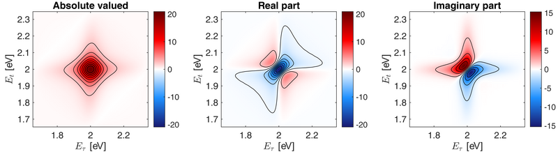
Here, the absolute-valued photon echo spectrum is displayed together with its real and imaginary part. A resonance appears at exactly (2.0, 2.0) eV which is identical to the system resonance we defined above.

Note: plotCMDS only represents an example plotting tool which allows you to get quick feedback of a simulation result and thus may lack more advanced data analysis functionalities in its current implementation. Of course, you can use your own customized evaluation and plotting tools. For that purpose, the raw simulation output (raw data matrix and time axes in femtoseconds), which you want to process with your own script, can be stored in the workspace by calling

1 2 3

resultCMDSdata = c.CMDSdata; tau_delay = c.delayAxes{1}/s.fstoau; t_delay = c.delayAxes{2}/s.fstoau;

The CMDS class is optimized to simulate population-based 2D spectroscopy and supports the simulation of two-, three- and four-pulse experiments in its current state.

References

[1] H.-S. Tan, Theory and phase-cycling scheme selection principles of collinear phase coherent multidimensional optical spectroscopy, J. Chem. Phys. 129, 124501 (2008).