1. Basics – Nlevel-Systems, Quantum Harmonic Oscillators and Couplings
In order to get started let us build a simulation for the example from the start page: two qbits which are coupled via a mode of the light field.
The three central entities of the toolbox are the System, Nlevel and Qoscillator classes.
The System class is a container class that contains all elements of one simulation. Every piece of QDT code starts with the declaration of a System object, which subsequently gets filled with all elements that are part of the simulation.
A Nlevel object represents a quantum system that – as the names suggests – has n discrete energy levels. The energy gaps between those levels are parameters of a Nlevel object.
A Qoscillator object represents a quantum-mechanical harmonic oscillator and can be used to model different bosonic excitations, like a mode of a light field or a plasmon in a cavity.
Nlevel and Qoscillator objects are often referred to as subsystems.
How does that look in practise for our example? Here is the code that implements a system of two qbits which are coupled via a mode of the lightfield.
1 | s = System; % create a System object |
Let us go through that line by line. In line 1, a System with the name s is created. We call it s just because that is short and we will have to call functions from the System class many times.
Next in line 2, the addentity function of the System class is called to add a subsystem to the simulation. This method takes two parameters, the subsystem that is to be added to the System object and a name by which we can henceforth address that subsystem. The Nlevel class takes a row vector that contains the energy differences between all levels of the subsystem. A [1] corresponds to a single energy gap of 1 a.u. (QDT runs entirely on atomic units) and thus a two-level system – a qbit. If we wanted to create a three-level system we would pass a three-level vector like [1 2]. The energy between the ground state and first excited state would be 1 a.u., the gap between first and second excited state 2 a.u.. Note that an energy gap of 1 a.u would corresponds to a transition in the extreme UV-range which is quite unrealistic for most experiments and used here just for simplicity.
Every function and class constructor in QDT is accompanied by a Matlab documentation providing examples and complete information on the possible syntax.
Line 3 is very similar to line 2. A quantum-mechanical harmonic oscillator is added to the simulation. The Qoscillator class takes two parameters: the number of levels which are simulated (this should be chosen so that the highest level has a low population at all times; a real quantum-mechanical harmonic oscillator has an infinite number of levels) and the energy gap between those levels (which must be a scalar since all levels are equidistant). Again, a value of 1 a.u. is chosen so that the subsystems are resonant.
In line 4, a second qbit is added to the simulation.
Now all that is missing are the dipole-dipole coupling terms. To add those the System class provides an addCoupling method that takes the names of the subsystems that are to be coupled and the coupling strength as parameters.
And now we are done. Six lines of code (five if you don’t count the first one) is all that is needed. Every element of the pen and paper version corresponds to one line of code. To run the simulation all we have to do is to set a time step and a maximum simulation time and run the simulate command of the System class and the density matrix for every time step will be calculated and stored within a variable called rho_hist inside the System class object s. Here is the complete code:
1 | clear; close all; |
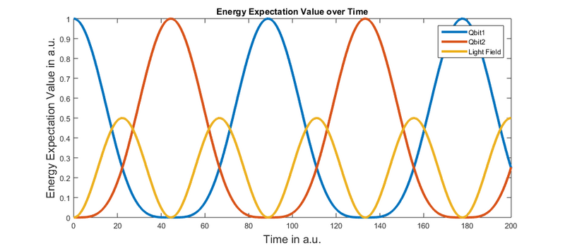
setState sets qbit1 in an excited state at the beginning of the simulation. Otherwise all subsystems were to start in the ground-state and since we have not added an external laser pulse to the simulation nothing would happen.
The System class provides a number of function to analyze the results of a simulation. The code